How to Add a Title to a Chart in Excel

How to Add a Title to a Chart in Excel

When creating a chart in Excel, you will normally want to add a title to your chart so the users better undertand the information contained in the chart. This tutorial will teach you how to add and format a title on your Excel chart.

Step 1: Click on a Chart Title

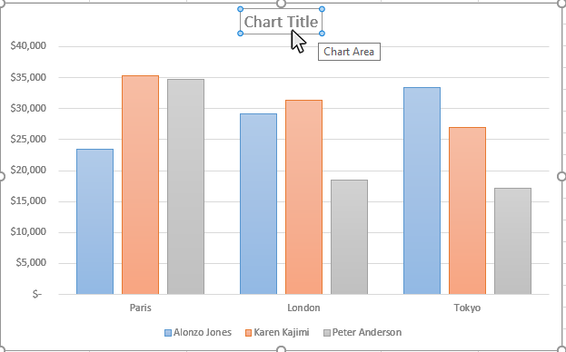
Use the cursor to click on a the "Chart Title" text on your chart. The border around the chart title area will become highlighted. Once you see the border appear around the chart, then you know it is ready to be changed.

Step 2: Type in the Name of the Chart

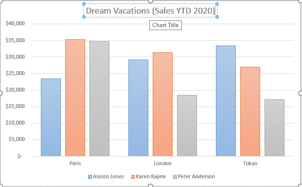
Once the chart name area is highlighted, you can type in the name of the chart. If you are happy with the look of the chart title, just click on a different part of the chart or worksheet and you will be done. If you want to do additional formatting to the chart, the next steps will show you how to do this.

Step 3: Format the Chart Title

There are a number of options to format your chart title. To access the formatting tools, double-click the chart title area on your chart. You are able to format your chart title in the following ways:

• Resize the Chart Title Area
• Reposition the Chart Title Area
• Change the Font Type
• Change the Font Size
• Change the Font Color
• Format the Chart Font (Bold, Italics, Underline)
• Change the Fonty Alignment (Left, Center, Right)

Topic #6

How to Add a Legend to a Chart in Excel

Thanks for checking out this tutorial. If you need additional help, you can check out some of our other free Excel Chart tutorials, or consider taking an Excel class with one of our professional trainers.